Overview

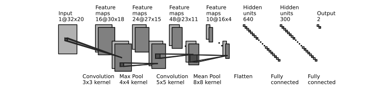
In this tutorial, we'll explore the key components of a convolutional neural network (CNN).

Outcomes

• Describe the components of a convolutional neural network
• Calculate the result of a convolution
• Calculate the result of max pooling
• Calculate the result of mean pooling

Introduction

In the previous unit, we built models that connect every input feature to each unit in a layer. These fully connected feed forward networks can learn complex relationships, but they do not explicitly favor nearby input positions or reuse the same feature detector at different positions.

For example, we could flatten an image into a vector and pass it to an MLP. Flattening does not destroy the pixel values or their ordering. What the MLP lacks is an explicit assumption that neighboring pixels belong together and that a useful pattern might appear in more than one location.

A convolutional neural network (CNN) makes that assumption part of its architecture. A filter examines a local window and reuses the same weights as it moves across the input. For text, those windows can contain neighboring characters or words. Later layers can combine the resulting features into more complex patterns.

Motivation

Convolutional neural networks arose from work in computer vision and drew inspiration from visual processing in the brain. The general idea is that an image is first built up from simple structures that are combined to form progressively more complex components.

These features are contextual (they depend on surrounding features) and hierarchical (simpler/more general features are composed to form more complex features).

Convolutional neural networks apply a series of convolutions to learn a hierarchy of context-dependent features.

For instance, if you wanted to learn to recognize images of cats, you might start with features encoding the pixel intensity in local regions of the image. Patterns in regional pixel intensity could be used to learn to detect edges. Edges might lead to detecting a cat's ear or the curve of a tail:

A similar, bottom-up approach could be used to learn to classify the language in which a document is written. One might start with sequences of characters and learn to identify patterns that approximate morphemes. Then, patterns in the sequences of coarse morphemes might reveal possible structures of words. Relations between words might reveal grammatical features:

Let's look at the operations that make this possible.

Convolutions

A convolution is an elementwise multiplication and summation applied repeatedly over a fixed-size sliding window. It's one way of encoding a property (or properties) across regions of some input. In an image, a convolution might tell us whether each region is bright or not.

Use of convolutions with fixed parameters predate neural networks. Among other things, fixed-parameter convolutions can be used to sharpen or blur images. Prior to the advent of convolutional neural networks and efficient backpropagation, kernels for convolutions were manually engineered to do things like recognize handwritten zip codes. A convolution operation has the following components:

Typical structure of a CNN

A convolutional neural network is composed of series of layers involving convolution and pooling operations to derive feature maps:

input $\rightarrow$ $\ldots$ $\rightarrow$ (conv $\rightarrow$ activation? $\rightarrow$ pooling $\rightarrow$ activation?)+ $\rightarrow$ $\ldots$ $\rightarrow$ output

Let's examine the convolution and pooling layers in more detail.

Convolutional layers

A convolutional layer learns one or more filters. At each position, a filter multiplies the values in its window by its weights, sums the products, and optionally adds a bias. The same weights are used at the next position. This is weight sharing: moving the filter does not create a new set of parameters.

Each output value depends on a limited region of the input, its receptive field. Stacking layers can expand that region, so later features can depend on more of the original input.

A text convolution visual

The visual uses the word cat with start and end symbols, giving us ^cat$, two illustrative embedding channels, and one filter of width two^†. Here, ^ and $ are explicit symbols in the input sequence, not padding or regular expression syntax. They let a filter encounter the beginning and end of a word. The vectors and filter weights are fixed so that we can inspect the arithmetic; they were not learned from data. The filter spans both channels and moves along character positions, not across embedding dimensions.

Examples

A convolution with a 1x3 kernel, stride of 1, and adjacent samples (PyTorch dilation=1):

A convolution with a 1x2 kernel, stride of 2, and adjacent samples (PyTorch dilation=1):

A convolution with a 2x2 kernel, stride of 1, and one gap between sampled positions (PyTorch dilation=2):

How many learnable parameters does a convolutional layer have?

Count the weights in one filter first. For a standard 1D convolution, a filter with width $k$ sees $C_{\text{in}}$ input channels, so it needs $C_{\text{in}} \times k$ weights. If it has a bias, add one more parameter^†. With $C_{\text{out}}$ filters, the layer has …

$$C_{\text{out}} \times (C_{\text{in}} \times k + 1)$$

For a standard 2D convolution, replace $k$ with the kernel's height times its width:

$$C_{\text{out}} \times (C_{\text{in}} \times k_h \times k_w + 1)$$

These counts assume groups=1 and a bias for each filter. Without biases, omit the + 1. The earlier shortcut, kernel size plus one, applies only to one filter with one input channel.

Pooling

Pooling summarizes values in a feature map, for example by selecting their maximum or calculating their mean. We can pool over local windows or over the entire sequence. Unlike a convolutional layer, these pooling operations have no learnable parameters.

Local pooling uses a window size and stride. PyTorch's max pooling also supports dilation; its average pooling layers do not expose a dilation argument. The average pooling animations below illustrate the arithmetic, including spaced windows, rather than an exact AvgPool configuration.

The most common forms of pooling are max and mean pooling.

Max Pooling

Max pooling selects the maximum value within a sliding window over some output.

Examples

Max pooling with a 2x3 window and adjacent samples (PyTorch dilation=1):

Max pooling with a 2x3 window and one gap between sampled positions (PyTorch dilation=2):

Mean Pooling

Mean pooling calculates the average within a sliding window over some output.

Examples

Mean pooling with a 2x3 window, a stride of 1, and adjacent samples:

Conceptual mean pooling with a 2x1 window, a stride of 1, and one gap between sampled positions. This illustrates the arithmetic, not an AvgPool dilation configuration:

How do CNNs relate to NLP?

It's easy to imagine and visualize how feature maps for an image relate to one another [2017], but its application to NLP may not seem so straightforward.

Linguistic information is both sequential and hierarchical. Consider the problem of learning to classify whether or not a document was written in Spanish or English. What information would be helpful in this task? We know that different natural languages place different constraints on the ordering of sounds, morphemes, and words. For example, if you randomly shuffled the characters of an English word, the result might not form a valid English word:

from random import shuffle

def scramble(word: str) -> str:
  symb = list(word)
  shuffle(symb)
  return ''.join(symb)

# this might return something nonsensical "lfdie"
# which wouldn't even qualify as a psuedoword in English
scramble('field')

The same holds true at the level of morphemes. pre + view forms a valid word in English (preview), but reversing the order of the combination (view + pre) fails this test (viewpre).

Meaning and grammaticality are both sensitive to order (both sequential and hierarchical structures). In order to reliably distinguish between English and Spanish, we need identify (or discover) the "fingerprints" or unique set of patterns that characterize each language.

Convolutions can provide a way of learning salient $n$-grams. Convolutions with dilations allow us to encode $n$-grams with gaps. Layers of such operations might allow us to learn more complex feature heirarchicies (ex. syntactic features).

A simple example

To further simplify, imagine we want to train a classifier to distinguish between Spanish and English words. In this problem setup, each word is a datapoint. Rather than use a bag of $n$-gram counts as our input, we'll encode each word as a matrix of character embeddings where each column stores the embedding for the character at that position in the word (ex. col 1 corresponds to char 1) and then apply a series of convolution and pooling operations over this matrix to learn featuring mappings. For the purpose of this example, assume that these character embeddings were learned via skip-gram, CBOW, or GloVe.

In the example above, a 2x2 convolutional kernel is applied to 5-dimensional character embeddings for words of 5 characters or fewer. In cases with fewer than 5 characters, padding is applied to the right edge of the word.

Imagine this operation is followed by a series (layers) of convolution, activation and pooling operations. In this way, one could construct a CNN for text classification.

Build a small CNN classifier

Let's connect this to the PyTorch models from the previous unit. We'll build a small character CNN with four steps:

1. Look up an embedding vector for each character ID.
2. Put embedding channels before sequence length and apply a shared filter bank.
3. Apply ReLU and keep the strongest activation for each filter.
4. Pass those pooled features to a linear classifier.

Unlike the older 2D example above, this Conv1d moves only along the character sequence. Each filter sees all four embedding channels^†. We will use two sequences of length five, with no padding, to keep the first forward pass easy to inspect.

import torch
from torch import nn

class TinyTextCNN(nn.Module):
    def __init__(self):
        super().__init__()
        self.embedding = nn.Embedding(12, 4)
        self.conv = nn.Conv1d(4, 3, kernel_size=2)
        self.classifier = nn.Linear(3, 2)

    def forward(self, ids):
        embedded = self.embedding(ids)           # (batch, length, channels)
        conv_input = embedded.transpose(1, 2)    # (batch, channels, length)
        features = torch.relu(self.conv(conv_input))
        pooled = features.max(dim=-1).values     # one value per filter
        return self.classifier(pooled)          # two class scores per example

# a -> 1, b -> 2, c -> 3; each row is one character sequence
ids = torch.tensor([[1, 2, 3, 1, 2], [3, 1, 2, 3, 1]], dtype=torch.long)
model = TinyTextCNN()
logits = model(ids)
print(logits.shape)  # torch.Size([2, 2])

Here is the shape of the data at each step:

Try inspecting these shapes yourself. Why does the convolution produce four positions from five input characters? Why does pooling leave three values per example?

CNN vs character n-grams

Recall our n-gram features. A character bigram classifier can count sequences such as ab, bc, and ca, then learn a classifier over those counts. A character CNN also examines short windows, but learns filters over embedding vectors rather than assigning a separate input feature to each exact bigram.

For a concrete comparison, inspect the bigram counts for the same two strings:

from sklearn.feature_extraction.text import CountVectorizer

vectorizer = CountVectorizer(analyzer="char", ngram_range=(2, 2), lowercase=False)
counts = vectorizer.fit_transform(["abcab", "cabca"])
print(vectorizer.get_feature_names_out())  # ['ab' 'bc' 'ca']
print(counts.toarray())                   # [[2 1 1], [1 1 2]]

Those counts are the input features, not predictions. A familiar classifier could be constructed as follows:

from sklearn.linear_model import LogisticRegression
from sklearn.pipeline import make_pipeline

bigram_classifier = make_pipeline(
    CountVectorizer(analyzer="char", ngram_range=(2, 2), lowercase=False),
    LogisticRegression(),
)

We have only constructed this classifier, just as we constructed the CNN. Neither has been trained in these examples. The bigram extraction rule is fixed, though its feature vocabulary is established from the training text and its classifier weights would be learned. In our CNN, the embeddings, filters, and final classifier weights would all be learned.

Compare the two classifiers in a few sentences:

• Which parts of each approach are learned, and which are fixed by our design?
• What does a bigram count retain that global max pooling discards? What order information is already lost by a bag of bigram counts?
• If the CNN scores a held-out example differently, would that alone show that it is better? What evaluation would you need?

For a performance comparison, both models would need training and evaluation with the same labels and data splits. Fit the n-gram vocabulary and any data-dependent preprocessing on the training split only. Architecture alone does not tell us which model will perform better.

A complex example

One of the early successes in applying deep learning to NLP used a convolutional neural network to learn to perform a series of progressively more complex foundational tasks. [2008] Remarkably, the approach uses very simple features as its input at a time when all of the state-of-the-art systems relied on hand-crafted features. Many of the ideas presented in that paper were so influential, they radically altered the course of research in the field for years.

If you're curious to delve deeper, the authors published a much more detailed follow up paper [2011].

Next steps

• CNNs in PyTorch: [The second half of Chapter 4 in Natural Language Processing with PyTorch](https://arizona-primo.hosted.exlibrisgroup.com/permalink/f/evot53/01UA_ALMA51631187280003843 ) [2019] walks through defining a CNN in PyTorch. Try following those steps to train your own CNN for the same problem. Next, try apapting it to work with a different dataset.

• Read A Unified Architecture for Natural Language Processing [2008], and try to summarize the approach in your own words. As you read this paper, Keep Andrew Ng's tips in mind (from 6:30 to 13:52 mark).

• Practice activities in Class Maestro

Practice

• For a convolution over a 10x6 input using a 2x3 kernel with a stride of 1 and a dilation of 1, calculate the dimensions of each output channel (feature map). Generalize this to a function for calculating the output of each channel/feature map given input dimensions, kernel dimensions, stride, and dilation.

• How does padding the input alter the dimensions of the output for a convolution or pooling operation? When might this be useful?

• A dilation allows comparisons with more distant contexts that are independent of immediate or local features. How might this be useful for problems involving human language?

• In the example of language identification for individual words, a matrix of character embeddings was proposed as input where each column $c_{i}$ encoded an embedding for the character at position $i$ in the word. Could the character embeddings be represented as rows instead of columns? If so, what might need to change?

References

- Olah, Chris and Mordvintsev, Alexander and Schubert, Ludwig (2017). Feature Visualization. Distill. 10.23915/distill.00007
- Rao, Delip and Mcmahan, Brian (2019). Natural language processing with PyTorch. O'Reilly Media github.com/delip/PyTorchNLPBook
- Ronan Collobert and Jason Weston (2008). A unified architecture for natural language processing. Proceedings of the 25th international conference on Machine learning - ICML 08. ACM Press 10.1145/1390156.1390177
- Ronan Collobert and Jason Weston and L\'eon Bottou and Michael Karlen and Koray Kavukcuoglu and Pavel P. Kuksa (2011). Natural Language Processing (Almost) from Scratch. Journal of Machine Learning. 2493--2537 Www.jmlr.org/papers/volume12/collobert11a/collobert11a.pdf