Overview

How might we represent a sequence while keeping track of what we've already seen? A recurrent neural network (RNN) updates a hidden state as it moves through the sequence. We'll follow those updates, connect them to PyTorch, and then look at gated RNNs and encoder-decoder architectures.

Outcomes

After completing this lesson, you'll be able to …

• trace how an RNN updates its hidden state across a sequence
• distinguish token IDs, embeddings, per-token outputs, and final hidden states
• explain the roles of LSTM gates and bidirectional context
• describe how an encoder and decoder map between sequences

Basic RNN

Many of the central tasks in natural language processing revolve around representing sequences.

We use these representations to do things like classify sequences, label elements in some sequences (POS tagging, NER, etc.), and map one sequence to another (translation, summarization, etc.). In earlier lessons, we saw networks that learn local patterns in sequences (ex. $n$-grams and $n$-grams with holes). Simple feedforward neural networks, such as an MLP that takes a flattened sequence as input, expect a fixed input size. They cannot directly accept sequences of arbitrary lengths without some way of making those inputs compatible (ex. padding, truncation, or pooling).

Since it lacks a memory mechanism that carries information from one timestep to the next, a simple feedforward network is not naturally suited to tracking a narrative or changes to the state of some world over time. Recurrent neural networks (RNNs) provide such a mechanism through their hidden state^†, which incorporates a "memory" of what has already been seen. This information helps contextualize the current input and influences how the state is updated. More abstractly, memories of the past contextualize our interpretation of the present and influence the formation of new memories.

The basic update is:

$$h_t = \tanh(W_{ih}x_t + b_{ih} + W_{hh}h_{t-1} + b_{hh})$$

Here, $x_t$ represents the current input and $h_{t-1}$ represents the previous state. The input and previous state have separate weight matrices. The same pair of matrices is reused at every timestep. Input vectors and hidden states need not have the same size.

This is an Elman network [1990], also called a vanilla RNN or simple recurrent network (SRN). A Jordan network uses a different recurrent connection, so those names aren't interchangeable.

Christopher Olah provides the following rolled and unrolled views:

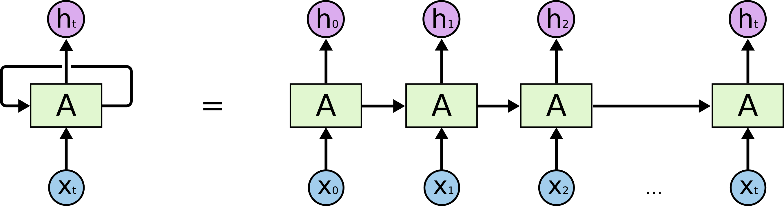
RNNs don't create a new set of parameters for every token, but instead apply the same update repeatedly through the sequence.

Follow the hidden state

Let's return to characters and use the word cat. At the first step, the network combines the embedding for c with an initial state. At the second, it combines a with the state produced after c. At the third, it combines t with the state produced after ca.

The labels describe which inputs have been processed. This is not a guarantee that the state remembers them perfectly. Reversing the character order changes the sequence of updates, even though the same character embeddings and parameters are used.

One step at a time in PyTorch

nn.RNNCell makes each update explicit. This example has four input features and six hidden features. The embeddings and recurrent weights are randomly initialized, so we're inspecting the computation, not claiming to have learned anything about cats.

import torch
from torch import nn

torch.manual_seed(42)

char_to_id = {"c": 0, "a": 1, "t": 2}
ids = torch.tensor([char_to_id[char] for char in "cat"], dtype=torch.long)
embedding = nn.Embedding(len(char_to_id), 4)
cell = nn.RNNCell(input_size=4, hidden_size=6)

# Start this independent sequence with no accumulated information.
h = torch.zeros(6)
states = []
for x_t in embedding(ids):
    h = cell(x_t, h)
    states.append(h)

cell_outputs = torch.stack(states)
print(cell_outputs.shape)  # torch.Size([3, 6])
print(h.shape)             # torch.Size([6])

Each row of cell_outputs is a state after one character. The final h is a representation after all three characters.

Let PyTorch handle the sequence

Rather than writing the loop ourselves, we can use nn.RNN. Let's put cat and act in a batch.

batch_ids = torch.tensor([[0, 1, 2], [1, 0, 2]], dtype=torch.long)
embedded = embedding(batch_ids)
rnn = nn.RNN(input_size=4, hidden_size=6, batch_first=True)

outputs, hidden = rnn(embedded)
print(embedded.shape)  # torch.Size([2, 3, 4])
print(outputs.shape)   # torch.Size([2, 3, 6])
print(hidden.shape)    # torch.Size([1, 2, 6])

We didn't pass an initial state, so PyTorch supplies zeros. outputs has one state per timestep for each example. hidden has the final state for each recurrent layer and direction^†. This new layer has its own randomly initialized parameters, so don't expect its numerical values to match our earlier cell's values.

From a sequence to a class

For a sequence classifier, we can pass the final state to a linear layer. This follows the same define -> predict pattern as our earlier classifiers.

import torch
from torch import nn

class RNNClassifier(nn.Module):
    def __init__(self, input_dim, hidden_dim, num_classes, num_layers=1):
        super().__init__()
        self.rnn = nn.RNN(
            input_size=input_dim,
            hidden_size=hidden_dim,
            num_layers=num_layers,
            batch_first=True,
        )
        self.fc = nn.Linear(hidden_dim, num_classes)

    def forward(self, x):
        _, hidden = self.rnn(x)
        # Use the final state from the top recurrent layer.
        return self.fc(hidden[-1])

classifier = RNNClassifier(input_dim=4, hidden_dim=6, num_classes=3)
logits = classifier(embedded)
print(logits.shape)  # torch.Size([2, 3]): examples, classes

The classifier returns raw scores (logits), not probabilities. For multiclass training, nn.CrossEntropyLoss accepts these scores and integer class labels directly. We don't apply softmax first.

Our examples so far have equal lengths and no padding. Before using this pattern with different lengths, read the padding discussion.

Applications of RNNs

We can use one final representation to classify a sequence, use per-token outputs to label its elements, or use a recurrent decoder to produce another sequence. Karpathy's visual illustrates these arrangements:

Encoder-Decoders

Suppose our input is a sentence in one language and our desired output is a sentence in another (i.e., a machine translation task). We don't necessarily have the same number of tokens on each side.

An encoder processes the source sequence. A decoder produces the target sequence. In a basic recurrent encoder-decoder, the encoder's final state initializes the decoder. The decoder then updates its own state while predicting target tokens.

During training, we often provide the previous correct target token as the next decoder input. This is called teacher forcing. During generation, that correct answer isn't available, so the decoder uses its own previous prediction. A mistake can affect subsequent steps.

The source representation can become a bottleneck: we're asking one fixed-size vector to convey everything the decoder needs. In the next unit, attention will give the decoder another way to consult source representations.

Limitations of SRNs

A simple RNN can process longer sequences without adding a new set of parameters at each step. That doesn't mean it can reliably learn every long-distance dependency.

Consider agreement in English:

The dolphins that traveled all the way to Miami from Havana each Thursday morning without fail are very friendly.

Useful information has to survive many state updates. During training, gradients also travel through those updates. Repeated multiplication can shrink or amplify them. An RNN can therefore struggle to learn which earlier information matters. This connects to our discussion of gradients in training tips.

Improving RNNs with gates

A Long Short-Term Memory (LSTM) network [1997] maintains both a cell state and a hidden state. Its gates control what to retain, what to add, and what to expose.

Using the notation in PyTorch's LSTM documentation:

$$i_t = \sigma(W_{ii}x_t + b_{ii} + W_{hi}h_{t-1} + b_{hi})$$ $$f_t = \sigma(W_{if}x_t + b_{if} + W_{hf}h_{t-1} + b_{hf})$$ $$g_t = \tanh(W_{ig}x_t + b_{ig} + W_{hg}h_{t-1} + b_{hg})$$ $$o_t = \sigma(W_{io}x_t + b_{io} + W_{ho}h_{t-1} + b_{ho})$$ $$c_t = f_t \odot c_{t-1} + i_t \odot g_t$$ $$h_t = o_t \odot \tanh(c_t)$$

The forget gate $f_t$ scales the old cell state^†. The input gate $i_t$ scales the new candidate values $g_t$ before they are added. The output gate $o_t$ controls how much of the transformed cell state is exposed in the hidden state. It doesn't directly erase the cell's memory.

You don't need to memorize these equations to use an LSTM. Focus on the routes information can take. Gates make selective retention easier to learn, but they don't promise perfect memory or eliminate every gradient problem.

Follow an LSTM cell value

Let's follow one coordinate of the cell state through a single update. The visual keeps the previous cell value and candidate fixed while we explore the gates. A real LSTM computes its gates from the current input and previous hidden state. Here, we set them ourselves to inspect their effects. The sliders include idealized values of 0 and 1 for fully closed and fully open gates.

GRUs

A Gated Recurrent Unit (GRU) uses a hidden state without a separate LSTM cell state. Its reset and update gates provide another way to control how old and new information are combined. See Cho and colleagues' original encoder-decoder paper.

An LSTM and GRU have similar input shapes, but their returned states differ: a GRU returns hidden, while an LSTM returns (hidden, cell). Swapping the layer name alone isn't enough if the surrounding code assumes one of these structures.

Stacking recurrent layers

Sequence length and layer count are different dimensions. A sequence of three characters still has three timesteps whether we use one recurrent layer or two. Each layer processes all three timesteps.

In a two-layer RNN, the first layer reads our input embeddings. The second reads the first layer's outputs. At timestep $t$, that second layer combines the first layer's current output $h_t^{(1)}$ with its own previous state $h_{t-1}^{(2)}$. It learns another transformation of the sequence, with its own parameters and its own evolving "memory". While it can be hard to imagine what those later layers might encode, you can think of them as learning higher order features (ways of combining earlier features)^†.

The subscript gives the timestep, and the superscript in parentheses gives the layer. Arrows between timesteps carry each layer's state forward. Arrows between layers pass the current output upward. We've omitted each layer's initial state to keep the diagram readable. These are two recurrent layers, not three layers for three characters.

Looking in both directions

For classifying a complete sentence, both earlier and later words can be useful^†. A bidirectional RNN runs separate forward and reverse recurrences and combines their representations.

Let's build a bidirectional GRU encoder. We'll prepare its token IDs just below.

The code below combines stacking recurrent layers with bidirectionality. Its num_layers=2 means two stacked layers, and bidirectional=True means each layer runs a forward and a reverse recurrence.

import torch
from torch import nn

class GatedRNN(nn.Module):
    def __init__(self, vocab_size, emb_dim, hidden_dim, padding_id,
                 num_layers=1, dropout_prob=0.2):
        super().__init__()
        self.embed = nn.Embedding(vocab_size, emb_dim, padding_idx=padding_id)
        self.dropout = nn.Dropout(dropout_prob)
        self.rnn = nn.GRU(
            emb_dim, hidden_dim, batch_first=True, bidirectional=True,
            num_layers=num_layers,
            # Recurrent dropout is between layers, so needs multiple layers.
            dropout=dropout_prob if num_layers > 1 else 0.0,
        )

    def forward(self, ids, lengths):
        embedded = self.dropout(self.embed(ids))
        # Lengths include real tokens and BOS/EOS, but not end padding.
        packed = nn.utils.rnn.pack_padded_sequence(
            embedded, lengths.cpu(), batch_first=True, enforce_sorted=False
        )
        packed_outputs, hidden = self.rnn(packed)
        outputs, _ = nn.utils.rnn.pad_packed_sequence(
            packed_outputs, batch_first=True, total_length=ids.shape[1]
        )
        # The top layer's final forward and reverse states.
        summary = torch.cat([hidden[-2], hidden[-1]], dim=1)
        return outputs, summary

For hidden size 6, each direction contributes six features. The combined summary has twelve. The final forward and reverse states are in hidden, not both at the last sequence position of outputs.

Preparing data

We'll reuse our earlier path: symbols -> integer IDs -> embedding vectors.

from collections.abc import Sequence

import torch

# Build this vocabulary from training examples, not validation/test examples.
training_examples = [["I", "like", "turtles"], ["turtles", "swim"]]
specials = ["<PAD>", "<UNK>", "<BOS>", "<EOS>"]
vocab = {symbol: index for index, symbol in enumerate(specials)}
for example in training_examples:
    for symbol in example:
        if symbol not in vocab:
            vocab[symbol] = len(vocab)

PAD_ID = vocab["<PAD>"]
UNK_ID = vocab["<UNK>"]

def prepare_datum(
    tokens: Sequence[str],
    max_len: int,
    pad_initial: bool = False,
) -> tuple[torch.Tensor, int]:
    """Map symbols to IDs, add boundary tokens, and pad."""
    ids = (
        [vocab["<BOS>"]]
        + [vocab.get(token, UNK_ID) for token in tokens]
        + [vocab["<EOS>"]]
    )
    if len(ids) > max_len:
        raise ValueError("Sequence exceeds max_len. Choose a truncation policy explicitly.")
    length = len(ids)
    padding = [PAD_ID] * (max_len - length)
    ids = padding + ids if pad_initial else ids + padding
    return torch.tensor(ids, dtype=torch.long), length

end_padded, length = prepare_datum(["I", "like", "tortoises"], max_len=7)
start_padded, _ = prepare_datum(["I", "like", "tortoises"], max_len=7,
                                pad_initial=True)
print(end_padded.tolist())    # [2, 4, 5, 1, 3, 0, 0]
print(start_padded.tolist())  # [0, 0, 2, 4, 5, 1, 3]
print(length)                # 5, including BOS and EOS

The unseen word tortoises maps to <UNK>. Both padding arrangements preserve token order. They put the unused positions in different places.

Padding in RNNs

Padding lets us stack different length examples in one tensor. It doesn't tell an RNN to skip those positions. Even with a zero padding embedding, recurrent weights and biases can update the state.

For an ordinary unidirectional RNN on end-padded data, the last output position may represent several padding updates after the real sequence ended. For a bidirectional RNN, padding can affect the reverse recurrence too.

Now let's encode a batch with different lengths:

prepared = [prepare_datum(tokens, max_len=7) for tokens in training_examples]
sequence_ids = torch.stack([ids for ids, length in prepared])
lengths = torch.tensor([length for ids, length in prepared], dtype=torch.long)

encoder = GatedRNN(len(vocab), emb_dim=4, hidden_dim=6,
                   padding_id=PAD_ID, num_layers=2)
encoder.eval()  # Disable dropout while we inspect the representations.
with torch.no_grad():
    token_outputs, summaries = encoder(sequence_ids, lengths)

print(sequence_ids.shape)   # torch.Size([2, 7])
print(token_outputs.shape)  # torch.Size([2, 7, 12])
print(summaries.shape)      # torch.Size([2, 12])

The per-token output is padded back to seven positions for convenience. Those added positions are not extra recurrent states. They're just zeros included to match the padded input length. The summary uses the final real states from both directions.

Are RNNs still a thing?

We've focused on simple RNNs, LSTMs, and GRUs, but the idea of carrying a "memory" through a sequence is still being explored. We won't discuss these newer architectures in great detail at this stage, but it's worth knowing what researchers are trying to improve and where these ideas have been used.

Two examples are:

• RWKV, which combines recurrent processing during generation with a formulation that allows parallel computation during training. It aims to make language modeling efficient without keeping an ever-growing collection of past representations in memory.
• State space models (SSMs), which carry information through structured state updates. Mamba makes those updates depend on the current input, allowing information to be selectively retained or forgotten. Its design also addresses how to compute those updates efficiently.

How is that different from a gated RNN?

LSTMs and GRUs already select what to retain or replace. Their gates depend on the current input and previous hidden state, so later gate calculations generally have to wait for that state. This can make training on long sequences costly. Libraries like PyTorch speed things up with batching and optimized GPU operations, but those optimizations don't remove the dependency between successive states.

Mamba offers a different route to efficient training. It transforms the previous state linearly^†, while making key parts of the update depend on the current input. This structure allows updates across a known sequence to be combined using a parallel computation called a scan. Mamba provides a way to retain selective memory while doing more of the training computation in parallel. Generating new tokens still happens one token at a time. The paper explicitly connects selection to gating.

What have these been used for? RWKV has been trained as a language model, including more recent multilingual models. The original Mamba paper [2023] demonstrates language modeling, audio modeling, and modeling DNA sequences.

The important thing to keep in mind is that there isn't a single architecture that is best for every task (some researchers continue to search for this El Dorado). New architectures are valuable because different designs can be better suited to different tasks, data, and computational constraints.

The ideas can also be combined. Jamba is a language model that mixes Mamba and transformer layers. That gives us a teaser for the next unit: attention mechanisms allow information from different positions to be selectively combined in a weighted fashion. Often architectural innovations combine what worked from prior architectures and serve as a bridging design.

Practice

In the practice activity for this unit, we'll work through token IDs, embeddings, recurrent updates, and state shapes in small steps. A full encoder-decoder is a useful extension, but don't feel that you need to build a translation system just to understand a hidden state.

Resources

• Chapters 14-17 of Yoav Goldberg's Neural Network Methods for NLP [2017]
• Understanding LSTM Networks (Olah, 2015)
• The Unreasonable Effectiveness of Recurrent Neural Networks (Karpathy, 2015)

Next steps

• Attention and Augmented Recurrent Neural Networks [2016]
• LSTM Tricks in Ruder's Deep Learning for NLP Best Practices
• Optional implementation extension: PyTorch's sequence-to-sequence translation tutorial

References

- Albert Gu and Tri Dao (2023). Mamba: Linear-Time Sequence Modeling with Selective State Spaces. 10.48550/arXiv.2312.00752
- Jeffrey L. Elman (1990). Finding Structure in Time. Cognitive Science. Wiley 179--211 10.1207/s15516709cog1402_1
- Sepp Hochreiter and J\"urgen Schmidhuber (1997). Long Short-Term Memory. Neural Computation. MIT Press - Journals 1735--1780 10.1162/neco.1997.9.8.1735
- Alex Graves (2013). Generating Sequences With Recurrent Neural Networks. ArXiv.
- Cho, Kyunghyun and van Merrienboer, Bart and Bahdanau, Dzmitry and Bengio, Yoshua (2014). On the Properties of Neural Machine Translation: Encoder-Decoder Approaches. arXiv 10.48550/ARXIV.1409.1259
- Goldberg, Yoav (2017). Neural Network Methods for Natural Language Processing. Morgan & Claypool Publishers ebookcentral.proquest.com/lib/uaz/reader.action?docID=4843762
- Ruder, Sebastian (2017). Deep Learning for NLP Best Practices. www.ruder.io/deep-learning-nlp-best-practices/
- Chris Olah and Shan Carter (2016). Attention and Augmented Recurrent Neural Networks. Distill. Distill Working Group 10.23915/distill.00001