Overview

In this lesson, we'll learn about the components of vectors, as well as some basic vector operations.

Outcomes

After completing this lesson, you'll be able to ...

describe vectors in terms of magnitude and direction
define scalar
add, subtract, multiply, and divide vectors
add, subtract, multiply, and divide vectors using a scalar

Vectors

Vectors can be thought of as n-dimensional points in space.

1D

If we decided to represent words using a single feature (ex. a sentiment score), we could represent them as 1D vectors:

x
0.5
0.75
0.9

"Vectors with a single dimension." — Vectors with a single dimension.

A single dimension is pretty limiting, though.

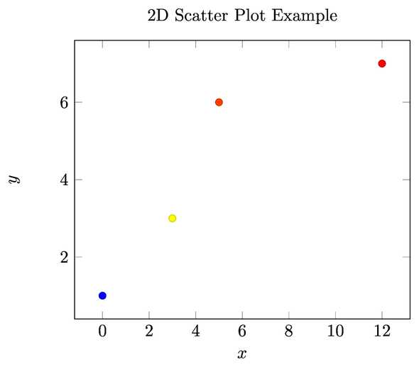
Even if we go beyond a single dimension, we can continue to think of vectors as points in n-dimensional space.

2D

x,y
0,1
12,7
3,3
5,6

"Vectors with 2 dimensions." — Vectors with 2 dimensions.

3D

x,y,z
0,1,2
12,7,5
3,3,3
5,6,6

"Vectors with 3 dimensions."

n-D

It's quite common to use 100s or 1000s of features (dimensions) to represent words and documents.

Beyond 3 dimensions, though, vectors become less straighforward to visualize. Some options include using properties such as color and shape to represent additional dimensions.

Properties of vectors

All vectors have two components:

length or magnitude
direction

Magnitude

The magnitude of a vector is its distance from the origin (i.e., the vector comprised of all zeros). Though it can be zero in a special case, length is never negative.

For a vector $\mathbf{a}$ , you'll often see $\| \mathbf{a} \|$ used to refer to its magnitude. If we're being more precise ¹, we'll use $\| \mathbf{a} \|_{2}$ to refer to the magnitude of $\mathbf{a}$ .

How do we calculate length? One familiar way of thinking about this is to consider a 2D vector and apply the distance formula to it and the origin. For this example, we'll consider the 2D vector $\mathbf{b} = \begin{bmatrix} 4 & 7 \end{bmatrix}$ :

\begin{aligned} d &= \sqrt{(4 - 0)^{2} + (7 - 0)^{2}} \\[2em] &= \sqrt{16 + 49} \\[2em] &= \sqrt{65} \\[2em] &\approx 8.06 \\[2em] \|\mathbf{b} \|_{2} &\approx 8.06 \end{aligned}

A 3-dimensional point (vector) will work the same way as will any $n$ -dimensional vector.

Norm

To calculate the magnitude (aka 2-norm) of any vector, we can use the following form of the distance formula:

\| \mathbf{x} \|_{2} = \sqrt{\sum_{i=0}^{\vert \mathbf{x} \vert} x_{i}^{2}}

Unit vector

The unit vector

A vector with a magnitude of 1 is called a unit vector.

Mathematical symbols: $\vert \mathbf{x} \vert$

What does $\vert \mathbf{x} \vert$ mean?

$\vert \mathbf{x} \vert$ is a way of specifying the cardinality or size of the vector $\mathbf{x}$ . For instance, if $\mathbf{x} = [0, 1, 1]$ , then $\vert \mathbf{x} \vert = 3$ .

Let's look at an example using Python.

Open the iPython REPL using a Docker container:

docker run -it "parsertongue/python:latest" ipython

x = [1, 2, 3, 4, 5]

cardinality = lambda vec: len(vec)

assert cardinality(x) == 5

Exit the iPython REPL and terminate the docker container:

exit

Mathematical symbols: $\Sigma$

What does $\Sigma$ mean?

The $\Sigma$ ("sigma") symbol is just a way of denoting a summation. For instance, $\sum_{i=0}^{\vert \mathbf{x} \vert}x_{i}$ simply means to sum all number in a vector $x$ from the 0 index until the last element of the vector.

Let's look at an example using Python.

Open the iPython REPL using a Docker container:

docker run -it "parsertongue/python:latest" ipython

x = [1, 2, 3, 4, 5]

sigma = lambda vec: sum(vec)

assert sigma(x) == 15

Exit the iPython REPL and terminate the docker container:

exit

Direction

The other component of a vector is its direction.

To calculate direction, we need to normalize a vector $\mathbf{x}$ by $\|\mathbf{x}\|_{2}$ . We do this by dividing each element $x_{i}$ of $\mathbf{x}$ by $\|\mathbf{x}\|$ . As an example, consider again the 2D vector $\mathbf{b} = \begin{bmatrix} 4 & 7 \end{bmatrix}$ :

\begin{aligned} \mathbf{b} &= \begin{bmatrix} 4 & 7 \\ \end{bmatrix} \\[2em] \|\mathbf{b} \|_{2} &\approx 8.06 \\[2em] \frac{\mathbf{b}}{\|\mathbf{b} \|_{2}} &= \begin{bmatrix} \frac{4}{\|\mathbf{b} \|_{2}} & \frac{7}{\|\mathbf{b} \|_{2}} \\ \end{bmatrix} \\[2em] \text{norm}(\mathbf{b}) &\approx \begin{bmatrix} 0.496 & 0.868 \\ \end{bmatrix} \end{aligned}

This resulting vector is known as a unit vector. It contains information solely about the direction of the vector.

We can can simplify the formula for normalizing a vector $\mathbf{x}$ as ...

\text{norm}(\mathbf{x}) = \frac{\mathbf{x}}{\| \mathbf{x}\|_{2}}

Operations

We can perform operations such as addition, subtraction, multiplication, and division on a vector and a scalar or a vector and another vector.

Scalar and vector

What is a scalar?

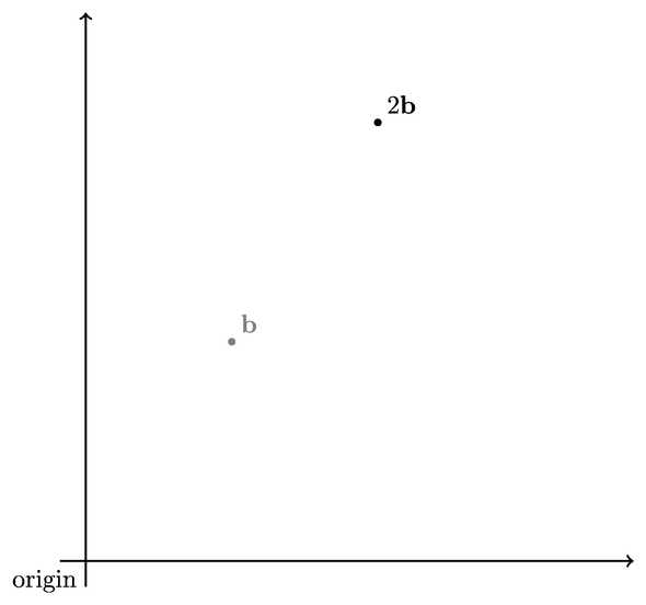
A scalar is a number that scales a vector.

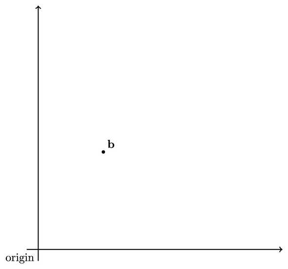
Say we have a two dimensional vector, $\mathbf{b}$ :

\mathbf{b} = \begin{bmatrix} 2 & 3 \\ \end{bmatrix}

We can visualize it as a single point:

"2D vector b." — 2D vector **b** (unscaled).

If multiply this vector by the scalar 2, we get the following result:

\begin{aligned} 2 \begin{bmatrix} 2 & 3 \\ \end{bmatrix} &= \begin{bmatrix} 2 \times 2 & 2 \times 3 \\ \end{bmatrix} \\[2em] &= \begin{bmatrix} 4 & 6 \\ \end{bmatrix} \end{aligned}

"2D vector 2b (scaled)." — 2D vector **2b** (scaled).

Vector and vector

Vector-vector operations rely on the two vectors having the same shape (dimensionality). These operations are performed against pairs of elements in the two vectors that share the same position (index). Let's look at a couple of examples ...

Subtraction

\begin{bmatrix} a \\ b \\ c \\ \end{bmatrix} \cdot \begin{bmatrix} d \\ e \\ f \\ \end{bmatrix} = \begin{bmatrix} a - d \\ b - e \\ c - f \\ \end{bmatrix}

Using NumPy

Invoke the IPython interpreter via docker:

docker run -it "parsertongue/python:latest" ipython

# run using the following command:
# docker run -it "parsertongue/python:latest" ipython

import numpy as np

x = np.array([1, 2, 4])
y = np.array([3, 4, 3])

x - y

The result:

np.array([-2, -2, 1])

Multiplication

\begin{bmatrix} a \\ b \\ c \\ \end{bmatrix} \times \begin{bmatrix} d \\ e \\ f \\ \end{bmatrix} = \begin{bmatrix} a \times d \\ b \times e \\ c \times f \\ \end{bmatrix}

Using NumPy

Invoke the IPython interpreter via docker:

docker run -it "parsertongue/python:latest" ipython

# run using the following command:
# docker run -it "parsertongue/python:latest" ipython

import numpy as np

x = np.array([1, 2, 4])
y = np.array([3, 4, 3])

x * y

The result:

np.array([3, 8, 12])

Next steps

You now know some basic vector operations. Before moving on to learning about comparing vectors, let's practice ...

Practice

Given $\mathbf{a} = \begin{bmatrix} 12 & 30 \end{bmatrix}$ , what is its magnitude?
Given $\mathbf{a} = \begin{bmatrix} 2 & 3 \end{bmatrix}$ , what vector has the same direction, but 3 times the magnitude of $\mathbf{a}$ ?
Given $\mathbf{a} = \begin{bmatrix} 2 \end{bmatrix}$ , what vector has the same magnitude, but the opposite direction to $\mathbf{a}$ ?

Footnotes

You'll learn why in the next lesson ↩

Overview

Outcomes

Vectors

1D

2D

3D

n-D

Properties of vectors

Magnitude

Norm

Unit vector

The unit vector

Mathematical symbols: ∣x∣\vert \mathbf{x} \vert∣x∣

What does ∣x∣\vert \mathbf{x} \vert∣x∣ mean?

Mathematical symbols: Σ\SigmaΣ

What does Σ\SigmaΣ mean?

Direction

Operations

Scalar and vector

What is a scalar?

Vector and vector

Subtraction

Using NumPy

Multiplication

Using NumPy

Next steps

Practice

Footnotes

Mathematical symbols: $\vert \mathbf{x} \vert$

What does $\vert \mathbf{x} \vert$ mean?

Mathematical symbols: $\Sigma$

What does $\Sigma$ mean?